基本信息
背景
为了挖掘结构化的信息,我们希望能得到节点的一个表示,其包含了图的结构信息。GraphSAGE 。
因此,本文提出了一种基于注意力机制的图分类网络。
实现方法
最主要的部分,self-attention层,其与Transformer中的self-attention机制相似,但是简化了很多:如果将Transformer中的self-attention机制中的Q、K、V全部认为是一样的,即共享参数,那么就能得到这篇文中的实现机制。
记节点i的特征为h i h_i h i
e i j = Feedforward ( W h i , W h j ) e_{ij}=\text{Feedforward}(Wh_i, Wh_j)
e ij = Feedforward ( W h i , W h j )
其中feedforward网络可以先用一个最简单的感知机实现:
Feedforward ( w 1 , w 2 ) = LeakyRelu ( a ⋅ concat ( w 1 , w 2 ) ) \text{Feedforward}(w_1, w_2)=\text{LeakyRelu}(a\cdot\text{concat}(w_1,w_2))
Feedforward ( w 1 , w 2 ) = LeakyRelu ( a ⋅ concat ( w 1 , w 2 ))
对于特定节点i i i
α i j = softmax j ( e i j ) \alpha_{ij}=\text{softmax}_j(e_{ij})
α ij = softmax j ( e ij )
最终,节点聚合的信息如下(只需要聚合一阶邻居的信息即可):
h i = ∑ j ∈ N ( i ) α i j W h j h_i=\sum_{j\in N(i)}\alpha_{ij}Wh_j
h i = j ∈ N ( i ) ∑ α ij W h j
为了进一步提升性能,还可以使用多头注意力机制,将最终的结果拼接或平均,得到最终结果。
如图所示:
为了得到更多的结构信息,还可以将多个self-attention层叠在一起,得到更多信息。(和GraphSAGE的K K K
优势
相较于GCN,不需要进行谱分解,并且可以并行计算。
分析W W W
只需要邻居的信息,无需全局信息,减少计算量
相较于GraphSAGE,可以采样所有的邻居,并且不存在LSTM处理无序序列带来的问题。(感觉有点故意拉踩了,GraphSAGE明明说的是防止计算量过大才采样邻居的,聚合器也提出了3种方法,池化方法性能也很强,该文非要逮着不太好的LSTM说)
实验结果
最终,无论是inductive还是transductive任务,都取得了很好的效果。
可解释性
不同颜色的节点代表不同的类别,边的粗细表示节点i和j之间的权重。
再通过降维技术,将其转化为2维,能直观的看到不同节点之间的关系。发现模型会关注 哪些信息。
代码阅读
source :https://github.com/Diego999/pyGAT
数据集结构
数据集为cora,是一个论文引用的图结构,包含两个部分:
content : 论文唯一标识符、特征、类别
cites : 论文引用关系
预处理数据集得到 邻接矩阵、特征、标签
模型结构
GraphAttentionLayer
先用了一个线性变换提取特征
1 Wh = torch.mm(h, self .W)
然后计算e i j e_{ij} e ij
Feedforward ( w 1 , w 2 ) = LeakyRelu ( a ⋅ concat ( w 1 , w 2 ) ) = LeakyRelu ( a 1 w 1 + a 2 w 2 ) \begin{aligned}
\text{Feedforward}(w_1, w_2)&=\text{LeakyRelu}(a\cdot\text{concat}(w_1,w_2))\\
&=\text{LeakyRelu}(a_1w_1+a_2w_2)
\end{aligned}
Feedforward ( w 1 , w 2 ) = LeakyRelu ( a ⋅ concat ( w 1 , w 2 )) = LeakyRelu ( a 1 w 1 + a 2 w 2 )
意味着这个前馈网络可以通过两部分相加实现,即
e i j = LeakyRelu ( a 1 W h i + a 2 W h j ) e_{ij}=\text{LeakyRelu}(a_1Wh_i+a_2Wh_j)
e ij = LeakyRelu ( a 1 W h i + a 2 W h j )
因此,利用pytorch的广播机制能很好地实现
[ a 1 W h 1 , a 1 W h 2 , ⋯ , a 1 W h N ] + [ a 2 W h 1 a 2 W h 2 ⋮ a 2 W h N ] [a_1Wh_1,a_1Wh_2,\cdots,a_1Wh_N]+
\left[\begin{matrix}
a_2Wh_1\\
a_2Wh_2\\
\vdots\\
a_2Wh_N\\
\end{matrix}\right]
[ a 1 W h 1 , a 1 W h 2 , ⋯ , a 1 W h N ] + a 2 W h 1 a 2 W h 2 ⋮ a 2 W h N
1
2
3
4
5
6
7
8
9
10
def _prepare_attentional_mechanism_input (self, Wh ): Wh1 = torch.matmul(Wh, self .a[:self .out_features, :]) Wh2 = torch.matmul(Wh, self .a[self .out_features:, :]) e = Wh1 + Wh2.T return self .leakyrelu(e)
然后创建掩码并计算(为了隐藏非相邻边的信息,在softmax时会被计算为0)
1
2
3
4
5
zero_vec = -9e15 *torch.ones_like(e) attention = torch.where(adj > 0 , e, zero_vec) attention = F.softmax(attention, dim=1 ) attention = F.dropout(attention, self .dropout, training=self .training) h_prime = torch.matmul(attention, Wh)
最终得到 N × feature N\times \text{feature} N × feature
GAT
首先是初始化函数,创建一个nheads个多头注意力,和一个输出层。其中GraphAttentionLayer的concat参数我觉得名字取得不好,因为这个参数是GAT的行为而不是GraphAttentionLayer的行为,当这个参数为True时,GraphAttentionLayer会在输出上应用一个激活函数。(并且,我觉得就不应该在GraphAttentionLayer内部实现激活函数,直接将激活函数移至GAT的forward函数中,这样能减少不必要的函数传参,更简洁)
1
2
self .attentions = [GraphAttentionLayer(nfeat, nhid, dropout=dropout, alpha=alpha, concat=True )self .out_att = GraphAttentionLayer(nhid * nheads, nclass, dropout=dropout, alpha=alpha, concat=False )
然后是forward函数
1
2
3
4
5
x = F.dropout(x, self .dropout, training=self .training) x = torch.cat([att(x, adj) for att in self .attentions], dim=1 ) x = F.dropout(x, self .dropout, training=self .training) x = F.elu(self .out_att(x, adj)) return F.log_softmax(x, dim=1 )
这代码写的简直是左脑搏右脑,中间层的声明GraphAttentionLayer需要应用激活函数,然后最后输出层out_att又声明不需要应用,然后在forward函数中又额外应用了elu激活函数。一点架构思想都没有。这应该还是参数名取得太差了,作者一看最后一层没有concat就把该参数设置为False,实际上GraphAttentionLayer根本不关心你是否要concat,换成use_elu,或者根本取消这个参数,都是很好的方法。
训练
1
2
3
4
5
6
7
8
9
10
11
12
13
14
15
16
17
18
19
20
21
22
23
24
25
for epoch in range (args.epochs): loss_values.append(train(epoch)) torch.save(model.state_dict(), '{}.pkl' .format (epoch)) if loss_values[-1 ] < best: best = loss_values[-1 ] best_epoch = epoch bad_counter = 0 else : bad_counter += 1 if bad_counter == args.patience: break files = glob.glob('*.pkl' ) for file in files: epoch_nb = int (file.split('.' )[0 ]) if epoch_nb < best_epoch: os.remove(file) files = glob.glob('*.pkl' ) for file in files: epoch_nb = int (file.split('.' )[0 ]) if epoch_nb > best_epoch: os.remove(file)
可以看到,这里使用了early stopping,当验证集上的损失不再下降超过一定次数时,就停止训练。torch.save os.remove),跑一个epoch(0.5s的样子)就io一下磁盘也是重量级。虽然对于固态硬盘来说IO的时间也很短,最后测下来也只有个位百分比的时间影响,但看着总是不太舒服。
这里的训练也没啥好说的,就是监督训练。不过值得注意的是,这里使用了F.nll_loss,这是负对数似然损失,这是因为在GAT中使用了log_softmax函数。(python中的crossentropy其实包括了log_softmax与nll_loss两部分)
1
2
3
4
5
6
7
8
9
10
11
12
13
14
15
16
17
18
19
20
21
22
23
24
25
26
def train (epoch ): t = time.time() model.train() optimizer.zero_grad() output = model(features, adj) loss_train = F.nll_loss(output[idx_train], labels[idx_train]) acc_train = accuracy(output[idx_train], labels[idx_train]) loss_train.backward() optimizer.step() if not args.fastmode: model.eval () output = model(features, adj) loss_val = F.nll_loss(output[idx_val], labels[idx_val]) acc_val = accuracy(output[idx_val], labels[idx_val]) print ('Epoch: {:04d}' .format (epoch+1 ), 'loss_train: {:.4f}' .format (loss_train.data.item()), 'acc_train: {:.4f}' .format (acc_train.data.item()), 'loss_val: {:.4f}' .format (loss_val.data.item()), 'acc_val: {:.4f}' .format (acc_val.data.item()), 'time: {:.4f}s' .format (time.time() - t)) return loss_val.data.item()